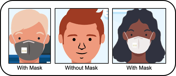
Face With/Without Mask classification using MobileNetV2

Jul 8, 2020 Deep learning, OpenCV, Raspberry Pi

Background

Corona Virus (COVID-19) has changed our daily lives and it is continuing to do so. As it kept going on for few months, in spite of presence of COVID-19, government has come up with reopening of stores and public places with various new regulations. One of the basic regulation being to wear face mask before entering any public places and following the social-distancing rules by staying 6 feet apart. In order to implement this many offices and public stores needed additional staff to guard doors to check if a person entering is wearing a mask or not.

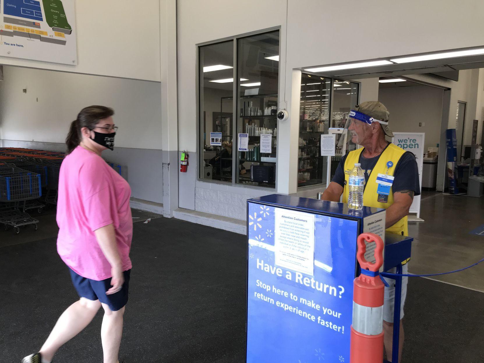
Walmart staff at entrance checking for masks [courtesy: poststar.com]

In order to overcome this, I decided upon building a Automatic Facemask detection system using available tools such as OpenCV, Keras, TensorFlow and deployed it onto a Raspberry Pi.

Dataset

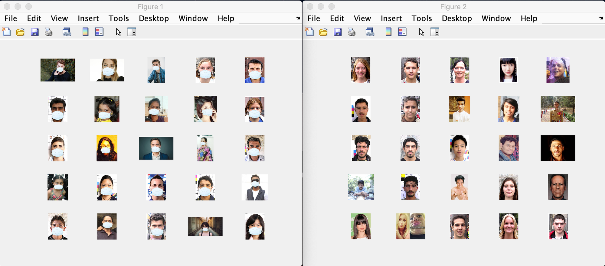
For building this model, I used the facemask dataset by Prajna Bhandary which has 1376 images with 690 images (with mask) and 686 images (without mask). In order to understand how was face mask dataset created, please refer to Adrain from Pyimagesearch.

Data Augmentation

After reading the dataset, the next step is to augment the dataset such that more number of images are available for training purpose. Here we use ImageDataGenerator from tensorflow.keras.preprocessing.image which takes batch of images and applies a series of random transformation (like rotation, shearing, resizing etc). Please note that, the ImageDataGenerator accepts the original data, randomly transforms it, and returns only the new, transformed data.

# Data Augmentation
aug = ImageDataGenerator(
	rotation_range=20,
	zoom_range=0.15,
	width_shift_range=0.2,
	height_shift_range=0.2,
	shear_range=0.15,
	horizontal_flip=True,
	fill_mode="nearest")

Split the data into train/test

Here we split, 80% of data into training set and 20% for testing. We use train_test_split from sklearn.model_selection with data and labels as input and outputs trainX, testX as training images & trainY, testY as categorical labels.

# split the data into 80% for training and 20% for testing
(trainX, testX, trainY, testY) = train_test_split(data, labels, test_size=0.20, stratify=labels)

Model definition

Here we will be fine-tuning the MobileNetV2 architecture, a very efficient architecture with limited computational capacity that can be applied on embedded devices such as Raspberry Pi, NVIDIA Jetson Nano, Google Coral etc. Fine-tuning is adapted to save the time taken to train the entire model.

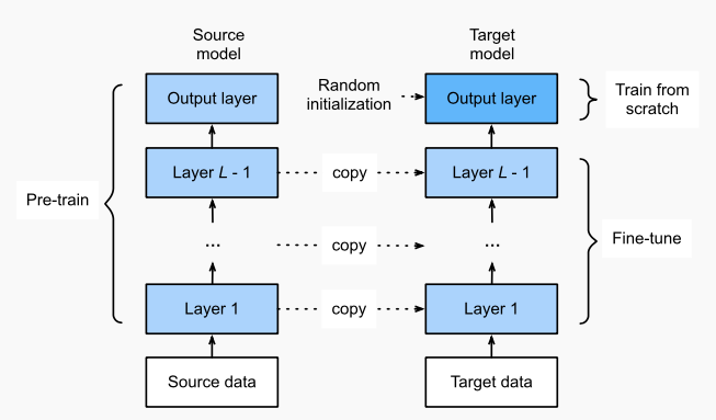
Fine-tuning is done for MobileNet by loading pre-trained ImageNet weights by leaving off the final layer (head) of the network and constructing a new fully connected layer that replaces the old one. As the weights of the old layers (other than just added fully connected layers) are with loaded weights, we freeze them and their weights are not updated during the backpropogation which means only the newly added ones gets trained.

# load the MobileNetV2 network without head layer
old_model = MobileNetV2(weights="imagenet", include_top=False)

# build a new FC layers
new_model = old_model.output
new_model = AveragePooling2D(pool_size=(7, 7))(new_model)
new_model = Flatten(name="flatten")(new_model)
new_model = Dense(128, activation="relu")(new_model)
new_model = Dropout(0.5)(new_model)
new_model = Dense(2, activation="softmax")(new_model)
model = Model(inputs=old_model.input, outputs=new_model)

# loop over all layers in old_model and freeze them not to train
for layer in old_model.layers:
	layer.trainable = False

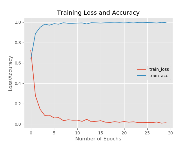
Training

We have data loaded up and model built, now we will move towards compiling and training our model to complete our task. Here we compile our model using Adam optimizer with initial learning rate of 0.0001 and decay depends on number of epochs. As its a binary model means detecting if face mask is present or not, we use ‘binary_crossentropy’ as a loss function. Then we use model.fit to train the model given its augmented data as input.

# compile our model
optmr = Adam(lr=0.0001, decay=0.0001 / num_of_epochs)
model.compile(loss="binary_crossentropy", optimizer=optmr, metrics=["accuracy"])
# train the unfrozen part of the network
mdl_trained = model.fit(aug.flow(trainX, trainY, batch_size=batch_size), epochs=EPOCHS)

Epoch 1/30
17/17 [==============================] - 33s 2s/step - loss: 0.7220 - accuracy: 0.6379
Epoch 2/30
17/17 [==============================] - 35s 2s/step - loss: 0.2780 - accuracy: 0.8880
Epoch 3/30
17/17 [==============================] - 34s 2s/step - loss: 0.1450 - accuracy: 0.9488
Epoch 4/30
17/17 [==============================] - 34s 2s/step - loss: 0.0846 - accuracy: 0.9807
Epoch 5/30
17/17 [==============================] - 33s 2s/step - loss: 0.0866 - accuracy: 0.9701
Epoch 6/30
17/17 [==============================] - 33s 2s/step - loss: 0.0601 - accuracy: 0.9846
Epoch 7/30
17/17 [==============================] - 34s 2s/step - loss: 0.0628 - accuracy: 0.9797
Epoch 8/30
17/17 [==============================] - 33s 2s/step - loss: 0.0334 - accuracy: 0.9942
Epoch 9/30
17/17 [==============================] - 33s 2s/step - loss: 0.0417 - accuracy: 0.9884
Epoch 10/30
17/17 [==============================] - 33s 2s/step - loss: 0.0376 - accuracy: 0.9884
Epoch 11/30
17/17 [==============================] - 33s 2s/step - loss: 0.0384 - accuracy: 0.9903
Epoch 12/30
17/17 [==============================] - 33s 2s/step - loss: 0.0260 - accuracy: 0.9923
Epoch 13/30
17/17 [==============================] - 33s 2s/step - loss: 0.0462 - accuracy: 0.9817
Epoch 14/30
17/17 [==============================] - 33s 2s/step - loss: 0.0227 - accuracy: 0.9952
Epoch 15/30
17/17 [==============================] - 32s 2s/step - loss: 0.0265 - accuracy: 0.9932
Epoch 16/30
17/17 [==============================] - 33s 2s/step - loss: 0.0330 - accuracy: 0.9903
Epoch 17/30
17/17 [==============================] - 33s 2s/step - loss: 0.0182 - accuracy: 0.9942
Epoch 18/30
17/17 [==============================] - 31s 2s/step - loss: 0.0156 - accuracy: 0.9952
Epoch 19/30
17/17 [==============================] - 33s 2s/step - loss: 0.0234 - accuracy: 0.9936
Epoch 20/30
17/17 [==============================] - 33s 2s/step - loss: 0.0170 - accuracy: 0.9952
Epoch 21/30
17/17 [==============================] - 34s 2s/step - loss: 0.0248 - accuracy: 0.9923
Epoch 22/30
17/17 [==============================] - 31s 2s/step - loss: 0.0180 - accuracy: 0.9961
Epoch 23/30
17/17 [==============================] - 32s 2s/step - loss: 0.0218 - accuracy: 0.9923
Epoch 24/30
17/17 [==============================] - 32s 2s/step - loss: 0.0147 - accuracy: 0.9971
Epoch 25/30
17/17 [==============================] - 32s 2s/step - loss: 0.0139 - accuracy: 0.9981
Epoch 26/30
17/17 [==============================] - 31s 2s/step - loss: 0.0167 - accuracy: 0.9961
Epoch 27/30
17/17 [==============================] - 32s 2s/step - loss: 0.0145 - accuracy: 0.9952
Epoch 28/30
17/17 [==============================] - 31s 2s/step - loss: 0.0196 - accuracy: 0.9913
Epoch 29/30
17/17 [==============================] - 32s 2s/step - loss: 0.0090 - accuracy: 0.9981
Epoch 30/30
17/17 [==============================] - 32s 2s/step - loss: 0.0124 - accuracy: 0.9952

Testing

Once the model is trained, we evaluate the model using the test dataset and finding the index of label with largest predicted probability and use classification_report from sklean.metrics view its well formatted classification report. Finally we save the model for future use.

predicted = model.predict(testX, batch_size=batch_size, steps_per_epoch=len(trainX)//batch_size, epochs=num_of_epochs)
pred_Idx = np.argmax(predicted, axis=1)
print(classification_report(testY.argmax(axis=1), pred_Idx, target_names=LabelBinarizer.classes_))
model.save(model_save_path, save_format="h5")

              precision    recall  f1-score   support

   with_mask       1.00      0.99      1.00       138
without_mask       0.99      1.00      1.00       138

    accuracy                           1.00       276
   macro avg       1.00      1.00      1.00       276
weighted avg       1.00      1.00      1.00       276

Summary

With the current results obtained, we see that the model is kind of performing overfitting which could be because of various reasons. Nevertheless, it is clear that with better and more data it is possible to train a model for face mask classification.

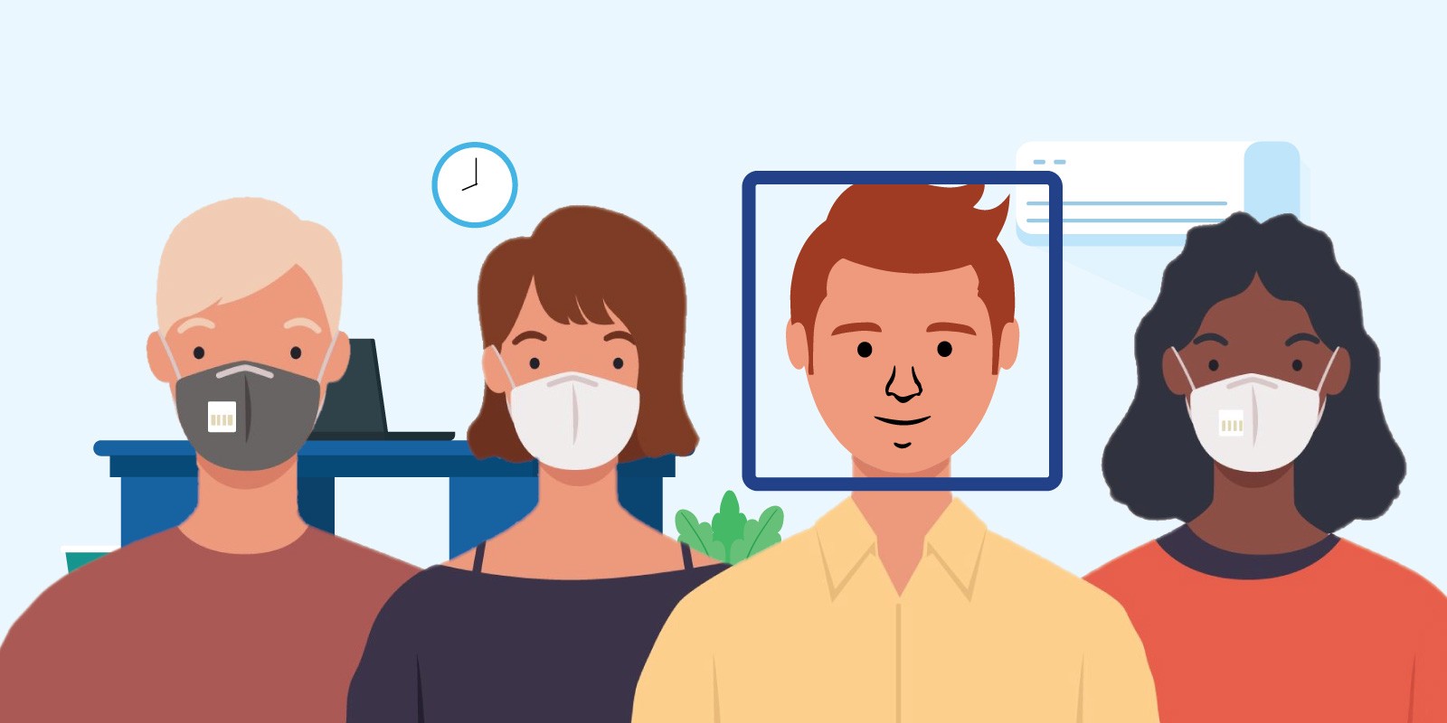
Now as the images were just the faces exposed to camera, the problem arises in taking it to real time where people need to get their faces closer to camera which in real time is not best method. In order to the model to work in real time we need to do the following:

Detect faces in given image/frame of video
Apply our current model (Face mask detecter) to the faces extracted from the image/frame.

Hence there is a need to train or use another model that detect faces given an image or frame from video as shown in figure below and then determine with or without mask. To read more about this implementation click here