EigenDigits - Eigenspace classification of Hand-Written Digits
Introduction
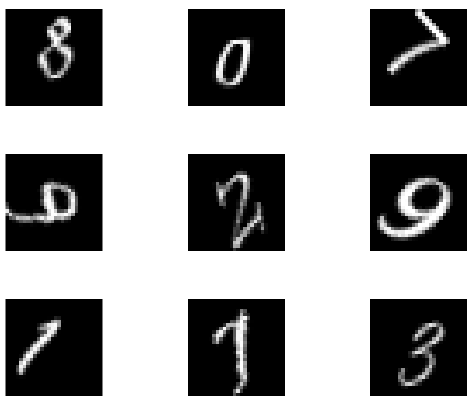
MNIST (Modified National Institute of Standards and Technology) database is a very large database with 60000 training images and 10000 testing images of handwritten digits. The database can be obtained from this url. This database is being used widely in the field of Machine Learning for training and testing purposes. This dataset contains normalized 28x28 pixel images in grayscale levels. Samples images are shown below.

In this project we classify the images from MNIST images using PCA and kNN as classifier. We project the data onto higher dimensional space and apply the concept of dimensionality reduction by selecting the eigenvalues and eigenvectors above the mean eigenvalue. Later, using the concept of kNN we find the distance between the vectors in eigenspace and classify the new vector’s label to the closest vector’s label. To achieve this we follow the algorithm discussed below.
Theory
In this task, we will compute the mean image and the principal components for a set of M training images that contain D pixels, i.e., $D=rows*columns=28^2$ for our MNIST images. For this project each test image is a training vector. We convert the training image with dimensions 28x28 to a feature vector, $\mathbf{\Gamma_i}$, by stacking each image column vertically in a single vector such that $\mathbf{\Gamma_i}$ has dimension $28^2$x1. If M is the total number of training images then the final input matrix or feature size will be $28^2$x$M$.
Computing the Principal Components of the Input Data
-
Read the set training feature vectors, $\Gamma$ $=$ ${\Gamma_1, \Gamma_2, …, \Gamma_M}$, from file and the associated label for each vector $\mathbf{L}={l_1, l_2, …, l_M}$ that indicate the correct labels for the handwritten digits in the corresponding images.
-
Compute $\mathbf{\Psi}$, the average image for all digits, from the values of each training vector, $\mathbf{\Gamma}_i$. Both $\mathbf{\Psi}$ and $\mathbf{\Gamma}_i$
will have dimensions D x1. $$ \Psi=\frac{1}{M} \sum_{n=1}^{M} \mathbf{\Gamma}_{n}$$
-
Compute the zero-mean version of each of the training images $\mathbf{\Phi}_i$ $=$ $\mathbf{\Gamma}_i - \mathbf{\Psi}$. Put all of the zero-centered training images into a D x M matrix $\mathbf{\Phi} = { \mathbf{\Phi}_1, \mathbf{\Phi}_2, …, \mathbf{\Phi}_M }$.
-
Compute C, the covariance matrix, using the zero-mean versions of the training images. $$ \mathrm{C}=\frac{1}{M} \mathbf{\Phi}^{t} \mathbf{\Phi} $$
-
Compute the principal components of the scatter matrix, C, and convert the resulting M eigenvectors, $\mathbf{v_i}$, of dimension M x 1 into M eigenvectors, $\mathbf{u_i}$, of dimension D x1. $$\mathbf{u_i}=\frac{1}{\left(M \lambda_{i}\right)^{1 / 2}} \mathbf{\Phi} \mathbf{v_i}$$
This will generate M eigenvectors, $\mathbf{u_i}$, which each have unit length, $\left|\mathbf{u}_{i}\right|^{2}=\mathbf{u_i}^{t} \mathbf{u_i}=1$, and dimension D x1. These eigenvectors span the eigenspace of the hand-written digits in the training images.
Dimensionality reduction and projecting the training data into the subspace (the eigenspace)
-
Compute the mean eigenvalue, $\bar{\lambda}=\frac{1}{M} \sum_{i=1}^{M} \lambda_{i}$, which we will use as a threshold for determining the subset of eigenvalues and associated eigenvectors which point in directions of significant image variation.
-
Form an eigenspace from the collection of eigenvalues and the associated eigenvectors which exceed the mean eigenvalue $\bar{\lambda}$. This will consist of K eigenvectors K<M which we can arrange as a set of columns in a matrix U with dimensions DxK.
$$ \mathbf{U}=\left[\begin{array}{llll}{\mathbf{u}_1} & {\mathbf{u}_2} & {\ldots} & {\mathbf{u}_K} \end{array}\right] $$
-
Compute the eigenspace representation for each of the training images by projecting each of the training images onto the $D$x$K$ subspace. This is equivalent to projecting each of the Dx1 zero-centered image vectors onto each of the K eigenvectors spanning the eigenspace. Each projection will generate a scalar result called a weight. We denote the weight computed by projecting training vector $\mathbf{\Gamma_m}$ onto eigenvector $\mathbf{u_k}$ as $\omega_{m,k}$. $$\omega_{m, k}=\mathbf{\Phi}{m}^{t} \mathbf{u}{k}=\left(\mathbf{\Gamma}{m}-\mathbf{\Psi}\right)^{t} \mathbf{u}{k}$$
The entire vector of K weights for the $m^{th}$ training vector may be computed as a row vector $\mathbf{\Omega_m}=\left[\omega_{m, 1}, \omega_{m, 2}, \ldots, \omega_{m, K}\right]$ in one matrix multiply using the following equation: $$ \mathbf{\Omega}{m}=\mathbf{\Phi}{m}^{t} \mathbf{U}=\left(\mathbf{\Gamma}_{m}-\mathbf{\Psi}\right)^{t} \mathbf{U} $$ which generates a 1xK dimensional vector of weights for training vector $m$. Finally, the whole collection of weights for all training vectors may also be computed in a single matrix multiply through the following equation: $$ \mathbf{\Omega}=\mathbf{\Phi}^{t}\mathbf{U} $$ where the $m^{th}$ row of the resulting $M$x$K$ matrix is the set weights $\mathbf{\Omega_m}$ for training vector $\mathit{m}$ .
Classification
Classification proceeds in a straightforward manner by projecting the zero-centered test vector into the eigenspace and performing a $\textit{k}$-nearest neighbour search within the eigenspace where $\mathit{k}$ =1.
-
Load a test image $\mathbf{\Gamma}_z$.
-
Convert this into a zero-mean image $\mathbf{\Phi_z}=\mathbf{\Gamma_z}-\mathbf{\Psi}$.
-
Project the test image into the eigenspace. $$ \mathbf{\Omega_z}=\mathbf{\Phi_z}^{\prime} \mathbf{U}=\left(\mathbf{\Gamma_z}-\mathbf{\Psi}\right)^{\prime} \mathbf{U} $$ This will generate a 1x$K$ vector of weights, $\mathbf{\Omega_z}=\left[\omega_{z, 1}, \omega_{z, 2}, \ldots, \omega_{z, K}\right]$, which is the dot product between each eigenvector, $\mathbf{u}_i$, and the zero-centered test image, $\mathbf{\Phi}_z$.
-
Find the eigenspace training vector closest to the projection of the test vector into the eigenspace $\mathbf{\Omega}_z$:
$$ \widehat{\mathbf{\Omega}}=\min _{1 \leq m \leq M}\left|\mathbf{\Omega}_m-\mathbf{\Omega}_z\right| $$
-
We then take as the classification for $ \mathbf{\Omega}_z $ the class label, $\hat{l}$, associated with the minimum distance training vector $\widehat{\mathbf{\Omega}}$.
Results
Now in order to understand the relationship between training images and accuracy for each alphabet we train our system with 5 training examples for each digit from the training data. Using the concepts discussed above we classified the first 3000 images from the test data. The output of classifier with error rates are shown below. We see that the classifier attained overall percent error of 43.13 i.e., 1706/3000 and time spent for classifications was 3.61 seconds.
| Digit | True Positive | Total Images | Percent Error |
|---|---|---|---|
| 0 | 167 | 271 | 38.38 |
| 1 | 305 | 340 | 10.29 |
| 2 | 161 | 313 | 48.56 |
| 3 | 170 | 316 | 46.20 |
| 4 | 205 | 318 | 35.53 |
| 5 | 50 | 283 | 82.33 |
| 6 | 222 | 272 | 18.38 |
| 7 | 205 | 306 | 33.01 |
| 8 | 149 | 286 | 47.90 |
| 9 | 72 | 295 | 75.59 |
Similarly, we trained with 10 training examples for each digit from the training data and first 3000 images from test data were chosen for classification. The output of classifier with error rates are shown below. We see that the classifier attained overall percent error of 35.60 i.e., 1932/3000 and time spent for classifications was 3.71 seconds.
| Digit | True Positive | Total Images | Percent Error |
|---|---|---|---|
| 0 | 194 | 271 | 28.41 |
| 1 | 335 | 340 | 1.47 |
| 2 | 182 | 313 | 41.85 |
| 3 | 252 | 316 | 20.25 |
| 4 | 222 | 318 | 30.19 |
| 5 | 64 | 283 | 77.39 |
| 6 | 211 | 272 | 22.43 |
| 7 | 205 | 306 | 33.01 |
| 8 | 166 | 286 | 41.96 |
| 9 | 101 | 295 | 65.76 |
Similarly, we trained with 20 training examples for each digit from the training data and first 3000 images from test data were chosen for classification. The output of classifier with error rates are shown below. We see that the classifier attained overall percent error of 28.70 i.e., 2158/3000 and time spent for classifications was 5.76 seconds.
| Digit | True Positive | Total Images | Percent Error |
|---|---|---|---|
| 0 | 224 | 271 | 17.34 |
| 1 | 335 | 340 | 1.47 |
| 2 | 190 | 313 | 39.30 |
| 3 | 257 | 316 | 18.67 |
| 4 | 231 | 318 | 27.36 |
| 5 | 116 | 283 | 59.01 |
| 6 | 207 | 272 | 23.90 |
| 7 | 205 | 306 | 33.01 |
| 8 | 190 | 286 | 33.57 |
| 9 | 203 | 295 | 31.19 |
Similarly, we trained with 30 training examples for each digit from the training data and first 3000 images from test data were chosen for classification. The output of classifier with error rates are shown below. We see that the classifier attained overall percent error of 23.00 i.e., 2310/3000 and time spent for classifications was 6.81 seconds.
| Digit | True Positive | Total Images | Percent Error |
|---|---|---|---|
| 0 | 245 | 271 | 9.59 |
| 1 | 337 | 340 | 0.88 |
| 2 | 198 | 313 | 36.74 |
| 3 | 246 | 316 | 22.15 |
| 4 | 239 | 318 | 24.84 |
| 5 | 185 | 283 | 34.63 |
| 6 | 226 | 272 | 16.91 |
| 7 | 226 | 306 | 26.14 |
| 8 | 182 | 286 | 36.36 |
| 9 | 226 | 295 | 23.39 |
Conclusion
After going through the results we analyzed the following.
- As the number of the training images increases, the overall error rate decreases. For number of training images = 30 and test images =3000, the overall error rate = 23%. Whereas for number of training images = 70 and same test images the overall error rate = 17.73%. So it decreases.
- When you increase the number of test images then you get approximately same overall error rate. For number of training images = 30 and test images = 3000 and 5000, the overall error rate is 23% and 23.20% respectively.
- Dimensionality reduction is the one of the beautiful concept. With K<M i.e., the number of images used as eigenspace is less than the number of images. Which is very helpful in decreasing the processing time. For N t =5 and M=10N t =60. The K was 16. Which is very less compared to M. Hence shows the dimensionality reduction.
- The loss of information or loss of energy by discarding or reducing dimension is very less and approximately the image is being reconstructed.
- K classifier is used which makes the classification process faster.
- Few digits such as 0 and 1 has more number of correct classifications when compared to others. 2,5,8 showed the most of error rate which means the training needs to be improved or use better algorithm.
Sunny Arokia Swamy Bellary
Research Engineer - Robotics
EPRI Engineer | AI Enthusiast | Computer Vision Researcher | Robotics Tech Savvy | Food Lover | Wanderlust | Team Leader @Belaku | Musician |